Abstract
The kernel trick is a powerful and versatile tool in machine learning applications. By utilizing the properties of mathematical kernel functions, we can transform data into different spaces where it can more easily be analyzed and understood. To effectively utilize the kernel trick, experts hand pick kernels a priori. The kernel’s hyper-parameters can then be tuned using a grid search over a region of interest. In this work, we model the kernel selection and hyper-parameter tuning as a single mixed integer nonlinear dynamics problem. As a result, we can eliminate the need for hand tuning the inputs. The system is shown to correctly select appropriate kernels in a handful of toy problems drawn from a combination of constant, liner, nonlinear terms.
INTRODUCTION
While neural networks on large server racks can crunch through billions of data points to train models, the method is infeasible when access to data or computing power is limited. Algorithms that utilize the kernel trick are more data efficient and so make sense for compact, mobile applications such as robots and mobile applications [@pmlr-v32-grande14]. Kernel methods also provide probabilistic outputs which correspond to a system’s certainty or uncertainty about an answer. In some situations, the resulting function can have a closed form solution and so do not suffer from the same local sup-optimal convergence problems that big data driven systems are prone to.
Kernel Functions
Positive definite kernel functions can be thought of as similarity transformations. Instead of transforming the data into a higher dimension to calculate the distance between two vectors, the kernel function can be used to directly compare vectors in the higher dimension without calculating the full transform. The goal in raising the data into a higher space is to allow it to be linearly separable.
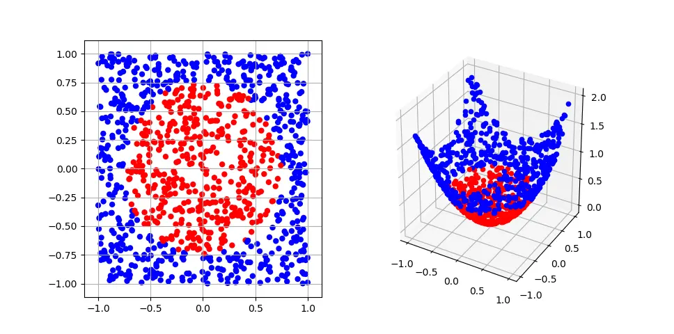
Consider we want to separate the data shown in the left graph in Figure 1 into two categories. On the 2D plane the data is far from linearly separable and so any efficient algorithms will fail. However, we can extend the data into a third dimension as shown in the graph to the right using the polynomial kernel, \[\label{eqn:kernel} k(x,y) = (x^Ty + c)^d.\] Here we see that the data can easily be separated by a hyper-plane in the higher space.
Mathematically, a positive definite kernel function \(k(\cdot,\cdot)\) is a symmetric function that satisfies, \[\sum\limits_i^n\sum\limits_j^n c_i c_j k(x_i,x_j) \geq 0, \quad x_{i,j} \in X, \quad c_{i,j} \in \mathbb{N}.\]
Kernel Regression
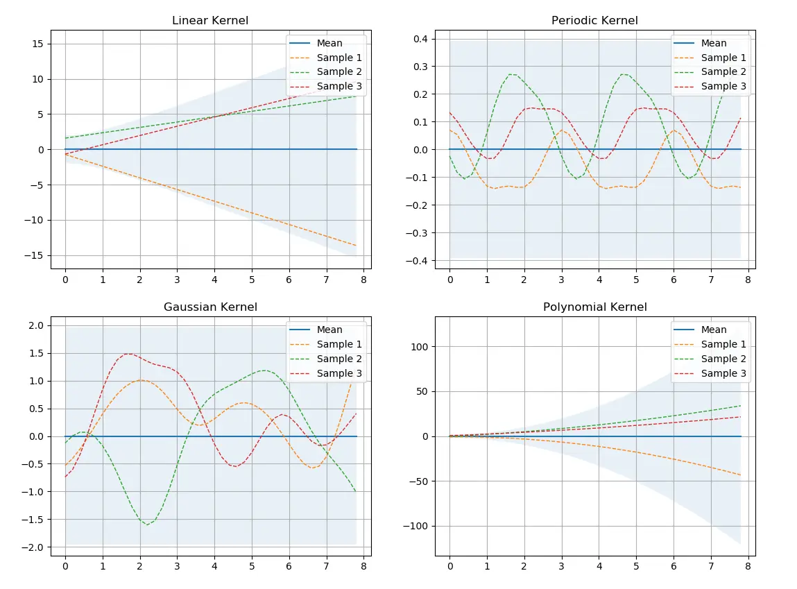
Aside from the classification example shown above, kernels can be used to perform a regression on data. A common technique to leverage the kernel trick for regression is the Gaussian process. Unlike parametric models which fit the parameters of a function to the given data, Gaussian processes generate a distribution directly over functions. Given a set of observations of an unknown function \(f = f(X)\), we assume data is drawn from a normal distribution of functions with some mean \(\mu\) and covariance \(\Sigma\), \[f|X \sim \mathcal{N}(\mu, \Sigma).\] Generally, the mean is taken to be the zero function to prevent the system from diverging. The kernel function is used to determine the general shape of the functions. We can see in Figure 2 how the choice of kernel function effects the pool of functions the system draws from. Because we have a probability distribution, we can sample from it to produce example functions. Each sub-graph in the figure shows three sample functions.
By assuming the functions are drawn from a normal distribution, we can take advantage of conditional and marginal distributions to extend the observations and make predictions. Given a set of new points \(y\) we can update the prior distribution \(p(f|X)\) by conditioning on the the set \(y\) to generate a posterior distribution, \(p(f|X,y)\). Furthermore, we can use the marginal distribution to make predictions \(f^*\) on hypothesized input data \(X^*\), \[p(f^*| X^*, X) = \int p(f^*|X^*,X)p(f|X) df.\] By the Gaussian assumption, the new distribution is also Gaussian. Specifically it can be given by the joint distribution, \[\begin{pmatrix} f \\ f^* \end{pmatrix} \sim \mathcal{N}\Big( 0, \begin{pmatrix} \Sigma_f & \Sigma^*_f \\ \Sigma_f^{*} & \Sigma^{**} \end{pmatrix} \Big).\]
The covariance matrices are given by plugging \(f\) and \(f^*\) into a chosen kernel function. \[\begin{aligned} k(f,f) & = \Sigma_f \\ k(f,f^*) & = \Sigma_f^* \\ k(f^*,f^*) & = \Sigma^{**} \end{aligned}\]
Log-Likelihood
The extent of this work is in the kernel optimization step of the learning process. To optimize the kernel we seek to solve the following problem: \[\begin{aligned} \max_\theta & \quad p(f|X)\\ \textrm{s.t.} & \quad f|X \sim \mathcal{N}(0, \Sigma) \end{aligned}\] where \(\theta\) is the set of hyper-parameters for a given kernel. In other words, we seek the parameters that maximize the the chance observing the data \(f(X)\).
One trick to simplify the calculation is to instead maximize \(\log p(f|X)\). Because the logarithm is a positive, increasing function, the optimization is equivalent. The log-likelihood function is given by \[\label{eqn:log} \begin{aligned} \log p(f|X) & = \log \mathcal{N}(0,\Sigma_f) \\ &= -\frac{1}{2}f^T\Sigma_f^{-1}f - \frac{1}{2}\log |\Sigma_f| - \frac{N}{2}\log 2\pi. \end{aligned}\]
As GAMs does not include built in methods for matrix inversions or determinants, much work was put into working around these limitations. The inversion of the covariance is a simple enough with two linear systems where we can enforce the following constraints on a separate variable, \(\hat{\Sigma}_f^{-1}\), \[\begin{aligned} \Sigma_f \hat{\Sigma}_f^{-1} & = I\\ \hat{\Sigma}_f^{-1} \Sigma_f & = I \end{aligned}\] To calculate the determinant we utilized the following relation, \[\label{eqn:det} |\Sigma_f| = |L|^2,\] where \(L\) is the Cholesky decomposition of the covariance matrix. The Cholesky decomposition is given by \[\label{eqn:eq} \Sigma = LL^*,\] where \(L\) is a lower triangular matrix. This decomposition only holds for positive definite Hermitian matrices. The matricies formed by positive definite kernel functions are symmetric by construction. However, in a misleading use of nomenclature, positive definite kernel functions produce positive semi-definite matrices. So long as we restrict the types of kernel functions the results hold. In GAMs, the implementation of the Cholesky decomposition requires two equations to compute. First, we enforce the equality given in equation [eqn:eq]. This requirement is simple enough with the introduction of a variable matrix \(L\). Second, we force the matrix to be lower triangular. From these four constraints we can obtain the determinant of the covariance matrix in equation [eqn:det].
Unfortunately, the above decomposition suffers from stability issues in all but trivial cases. We can instead use a predictive mean and variance derived from the Cholesky decomposition to address this shortcoming. To do so, we solve two systems of linear equations to derive the linear predictor form of the inverse system, \[\hat{x}_2 = L^T \backslash (L\backslash f).\] The above equation can be expressed in the form of two linear systems, \[L\hat{x}_1 = f,\] and \[L^T\hat{x}_2 = \hat{x}_1.\] The end result, \(\hat{x}_2\), is a linear approximation of the inverse calculation. The first term of equation [eqn:log] becomes \(\hat{x}^T_2 f/2\).
We can also simplify the second term in equation [eqn:log] into the Cholesky form using log power and log multiplication rules, \[\begin{aligned} \frac{1}{2}\log(|L|^2) & = \log(|L|)\\ & = \log(\prod_i L_{ii}) \\ & = \sum_i \log(L_{ii}) \end{aligned}\] where \(L_{ii}\) represents the \(i^{th}\) diagonal element of \(L\). The modified log-likelihood function is then given by, \[\log p(f|X)= -\frac{1}{2}\hat{x}^T_2 f - \sum_i \log(L_{ii}) - \frac{N}{2}\log 2\pi.\]
Mixed Integer Nonlinear Program
We are now ready to formulate the kernel selection and optimization problem as a mixed integer nonlinear program. Let \(\mathcal{K}\) be a set of kernels. Consider the following,
Lemma: The sum of two kernel functions is also a kernel function.
Proof: Let \(k_1\) and \(k_2\) be two kernel functions defined above in equation [eqn:kernel]. By construction, \(k_1\) and \(k_2\) are symmetric, hence, \[k_1(x,y) + k_2(x,y) = k_1(y,x) + k_2(y,x).\] Furthermore, the constant distribute over multiplication, \[\sum_i^n\sum_i^n c_i c_j (k_1 + k_2) = \sum_i^n\sum_i^n c_i c_j k_1 + c_i c_j k_2.\] As a result, we can rearrange the terms to create, \[\sum_i^n\sum_i^n c_i c_j k_1 + \sum_i^n\sum_i^n c_i c_j k_2 \geq 0.\] By construction each individual term in the summation is non-negative and so the total sum is also non-negative. Thus, \(k_1+k_2\) is a kernel function.
\(\square\)
For ever kernel function \(\Sigma_i \in \mathcal{K}\) create a binary variable \(b_i \in \mathcal{B}\). As a result let \(\Sigma^*\) be defined as follows, \[\Sigma^*_\theta = \sum_i b_i\Sigma_i.\] Let \(\theta\) represent the set of hyper-parameters associated with each kernel function. The MINLP can then be written as the maximization of the log likelihood term, \[\begin{aligned} \max_{\theta, \mathcal{B}} & \quad \log \mathcal{N}(0,\Sigma^*_\theta)\\ \textrm{s.t.} & \quad \Sigma^*_\theta = \sum_i b_i\Sigma_i \end{aligned}\]
PILCO
In the field of reinforcement learning, the main algorithm to utilize the Gaussian process is known as the Probabilistic Inference for Learning COntrol (PILCO). The objective is to use the probabilistic modeling capabilities of the GP to model the transition function of an unknown system for use in continuous control applications. The PILCO algorithm has been shown to learn control policies with orders of magnitude less data than comparable neural networks. As the objective of this work is to select a kernel for such applications PILCO’s mention here will remain brief.
ENVIRONMENT DATA
In many areas of machine learning toy environments have been constructed to be able to observe how different algorithms behave against specific scenarios. This provides a rich landscape from which we can draw data. The team at Open AI have released a public repository of a large selection of reinforcement learning environments [@brockman2016openai]. The two considered here are the continuous pendulum and continuous mountain car. Along side the more practical examples since kernel regression is designed to work as a black-box function approximate we can construct any number of mathematical functions from which we can draw data.
Black-box Functions
As the objective of a regression system is to model an unknown function, any constructed function can be used to test the limits of such a system. A simple test can be fitting to noisy linear trends. We can build upon this by adding non-linearities such as a periodic or polynomial components. From this we can determine the extent to which some kernels generalize. Furthermore, we seek to minimize the number of kernels a resulting model relies on. This is done by providing the optimization problem a handful of kernel functions which it can enable and disable as the optimization sees fit. We hope to see the system remove unnecessary kernel functions from the calculation to maintain efficiency.
Inverted Pendulum
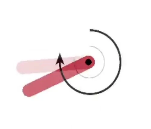
The inverted pendulum is a classical control problem with the objective of balancing a rotating rod at its unstable equilibrium. An example of the environment is shown in Figure 3 where the exerted torque is shown as an arrow.
The dynamics are known making the problem a good test to compare learning systems against optimal control models. The state space takes the form of a 3-tuple consisting of the cos and sin of the current angle, \(\theta\) of the rod and the current angular velocity of the rod, \(\dot{\theta}\). In order to act on the system, the agent can exert a bounded torque, \(\tau\) at the pivot point. To further constrain the search, the agent must also minimize the energy expended to stabilize the rod. The objective function is given by, \[J(\theta, \dot{\theta}, \tau) = -(\theta^2 + 0.1 b\dot{\theta}^2 + 0.001\tau^2).\]
Continuous Mountain Car
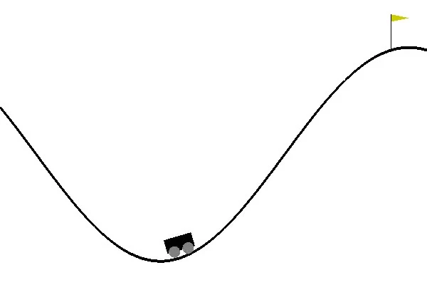
Another common example that highlights different challenges can be seen in the continuous mountain car environment. Here the agent controls a small car located in a 2 dimensional valley as shown in Figure 4.
The objective of this system is to get the car up the hill to the right. Doing so gets the agent a reward of 100, at all other time steps the reward is -1. Unlike the inverted pendulum, the mountain car environment has a sparse reward meaning an agent doesn’t know how close to the objective it is from the reward alone. The state space for this environment is a 2-tuple of the current position and velocity of the car. The action space is a bounded force exerted on the car, a negative value pushed the car left, positive to the right. To further increase the challenge of the environment, the car cannot directly drive up the hill to the right. The agent must learn a policy which first drives up the hill to the left to gain enough momentum to make it up the right hill. The sparsity of the reward function makes this especially challenging.
ANALYSIS
Due to the student license equation limit. The number of points that could be optimized over was greatly restricted. As a result, the only functions that could be tested where that of the black-box toy functions. To this end, the system successfully optimized the mixed integer nonlinear programs. The set \(\mathcal{K}\) consisted of the following kernels:
Constant Kernel: \[k_{const}(x,y) = \alpha\]
Linear Kernel: \[k_{lin}(x,y) = \beta \cdot x^Ty\]
Quadratic Kernel: \[k_{quad}(x,y) = (\gamma \cdot x^Ty)^2\]
Gaussian Kernel: \[k_{gaus}(x,y) = \sigma^2 e^{-\frac{1}{2len^2}(||x-y||^2)}\]
Given \(\mathcal{K}\), we can define the set \(\mathcal{B} = [b_1, b_2, b_3, b_4]\) where \(b_i \in \{0,1\}\) is a binary variable. Because the above lemma holds for any positive multiple of the kernel, we could consider the liner combination of kernels instead of binary variables. This, however, results in the need to calculate every kernel even if the underlying data is not described well by that particular kernel function. In order to avoid unnecessary calculations we let the system ’turn off’ kernels with the binary variables. The relative weights are then handled by the kernel function’s hyper-parameters. The total kernel function is given by the following formulation, \[\begin{aligned} k^* = b_1*k_{const} & + b_2*k_{lin} \\ + b_3*k_{quad} & + b_4*k_{gaus} + \sigma_f I_n. \end{aligned}\] The kernel hyper-perameters are given by \(\theta = (\alpha, \beta, \gamma, \sigma, l, \sigma_f)\). The last term, \(\sigma_f\), represents an estimation of the observation noise in the data. This term is included as a parameter of the total kernel function.
The optimization was run on four sets of noisy data drawn from a variety of underlying functions. The system then maximized the log-likelihood function over the observations.
Linear Function
The first set of data was drawn from the following linear function where \(\mathcal{N}(0, \sigma_f)\) is a zero-mean noise term, \[\label{eqn:linear_eqn} f(x) = 2x + 10 + \mathcal{N}(0, \sigma_f)\] The linear slope of \(2\) and constant offset of \(10\) where arbitrarily chosen. As seen in Table 1, the model correctly enabled the linear and constant kernel functions while disabling the quadratic and Gaussian kernels. Furthermore, it successfully converges to the system parameters with an appropriate noise estimation.
| Linear | |
|---|---|
| \(b_1\) | \(1.0\) |
| \(b_2\) | \(1.0\) |
| \(b_3\) | \(0.0\) |
| \(b_4\) | \(0.0\) |
| \(\alpha\) | 10.405 |
| \(\beta\) | 1.972 |
| \(\gamma\) | X |
| \(len\) | X |
| \(\sigma\) | X |
| \(\sigma_f\) | 0.432 |
Figure 5 shows the posterior mean calculated with the optimized parameters. The light blue area is the 95% confidence region calculated from the covariance matrix.
![Figure 5: Ten data points drawn from equation [eqn:linear_eqn] along side the output of the optimization.](/files/images/kernels/Test1.webp)
Quadratic Function
The second test introduced the first non-linearity in the form of a quadratic term.
\[\label{eqn:quad_eq} f(x) = \frac{1}{5}x^2 + 3 + \mathcal{N}(0, \sigma_f)\]
The GAMs model was successfully able to pick out the constant and quadratic terms while setting the binary variable associated with the linear and Gaussian terms to zero. The results of the second optimization are shown in Table 2.
| Quadratic | |
|---|---|
| \(b_1\) | \(1.0\) |
| \(b_2\) | \(0.0\) |
| \(b_3\) | \(1.0\) |
| \(b_4\) | \(0.0\) |
| \(\alpha\) | 3.205 |
| \(\beta\) | X |
| \(\gamma\) | 0.199 |
| \(len\) | X |
| \(\sigma\) | X |
| \(\sigma_f\) | 0.434 |
Figure 6 once again summarizes the posterior mean with it’s 95% confidence interval.
![Figure 6: Ten data points drawn from equation [eqn:quad_eq] along side the output of the optimization](/files/images/kernels/Test2.webp)
Polynomial Function
The third test ensured that the system would include all relevant kernels as opposed to dropping the linear term in favor of an incorrect quadratic slope.
\[\label{eqn_poly_eq} f(x) = \frac{1}{10}x^2 + 3x + 8 + \mathcal{N}(0, \sigma_f)\]
The GAMs model was successfully able to pick out the constant, linear and quadratic terms as shown by the \(b_i\) terms in Table 3 as well as determine the correct hyper-parameters associated with each kernel.
| Polynomial | |
|---|---|
| \(b_1\) | \(1.0\) |
| \(b_2\) | \(1.0\) |
| \(b_3\) | \(1.0\) |
| \(b_4\) | \(.0\)0 |
| \(\alpha\) | 8.381 |
| \(\beta\) | 2.937 |
| \(\gamma\) | 0.107 |
| \(len\) | X |
| \(\sigma\) | X |
| \(\sigma_f\) | 0.456 |
Figure 7 shows the posterior mean with it’s 95% confidence interval.
![Figure 7: Ten data points drawn from equation [eqn:poly_eq] along side the output of the optimization](/files/images/kernels/Test3.webp)
Larger Perturbations
Lastly, a larger, regular perturbation was introduced on top of a linear trend. The system successfully enabled the Gaussian kernel for this case instead of increasing the noise range to accommodate the change in data.
\[\label{eqn:nl_eq} f(x) = \sin(x) + \frac{1}{2}x + \mathcal{N}(0, \sigma_f)\]
The GAMs model was successfully able to pick out the linear and nonlinear terms as shown by the \(b_i\) terms in Table 4. Another observation is that, for reproduciblity, the noise remained constant through all the trials. The model accounted for this consistency with similar approximations of \(\sigma_f\) for each trial.
| Linear + Sin | |
|---|---|
| \(b_1\) | \(0.0\) |
| \(b_2\) | \(1.0\) |
| \(b_3\) | \(0.0\) |
| \(b_4\) | \(1.0\) |
| \(\alpha\) | X |
| \(\beta\) | 0.486 |
| \(\gamma\) | X |
| \(len\) | 1.536 |
| \(\sigma\) | 1.159 |
| \(\sigma_f\) | 0.511 |
Figure 8 shows the posterior mean with it’s 95% confidence interval.
![Figure 8: Ten data points drawn from equation [eqn:nl_eq] along side the output of the optimization](/files/images/kernels/Test4.webp)
CONCLUSION
Course Concepts
This work relied on an understanding of GAMs developed throughout this course. Furthermore, the project leveraged the the mixed integer nonlinear programs covered in the end of the semester.
Problems Encountered
While the project as a whole performed well, there are a few caveats that limit the usability of the system. The first is the aforementioned equation limit imposed by the student license. This restriction limited the number of data points the GAMs code would accept to under 15, well below the hundreds required to run a full reinforcement learning agent. The result is that the project serves as a proof of concept over a handful of test functions.
A second issue is the system’s sensitivity to the objective function and initial conditions. While the code converges rapidly for some function \(f(x)\), it will go on to return an infeasible result for \(f(x)+1\) and so on. Similarly, while an initial value of \(\alpha_0 = 0\) does not converge, a value of \(\alpha_0 = 1\) does. The sensitivity can be reduced by solving the system as a relaxed mixed integer nonlinear program, but this switch occasionally leaves some unnecessary kernel functions active.
Future Work
Both issues can be easily addressed. First, if the license is upgraded past the free version, the data limit will be removed. To account for the sensitivity of initial conditions, a sweep over these values can be implemented.