Written by Christopher Zawacki, Paul Reverdy, and D. E. Koditschek

The pdf can be downloaded here.

Abstract

Abstract—Gait synthesis and optimization is a key challenge in the field of legged robotics. The performance of the system often relies heavily on the parameters that define a gait. Increasing the number of parameters allows a gait to be more finely tuned but in turn increases the difficulty of the gait parameter optimization problem due to the curse of dimensionality. The dependence on a physical machine makes it costly to measure the performance of a given gait, and inconsistencies in the model such as motor heating and battery placement make the optimization process susceptible to noise. In this paper we demonstrate a new method for tuning parameters based on formulating the gait optimization problem as a multiarmed bandit problem. The method is designed to account for uncertainty resulting from measurement noise while requiring a low number of physical trials. We tested this method on QRHex, a quadrupedal, RHex-style robot with one actuator per limb. With this method we were able to decrease the cost of transport by 36.6%.

Introduction

Finding a gait for a legged robot is a challenging task even for an expert with extensive experience. Generally, the tuning process is reduced to a parameter optimization problem by adopting a parametric representation of admissible gaits. For RHex-style robots with one actuator per limb, a common approach to this reduction is to use a Buehler clock [20]. An expert can roughly tune the values of each gait parameter for a given situation using intuition, but the finer details are regularly tuned through exhaustive testing. One could quantify the relevant aspects of gait quality through an understanding of the physical system, thereby formulating a function that encodes the desirability of a gait. While this method produces an optimization problem that can be systematically solved, the resulting gait space increases exponentially in size with the number of gait parameters. This causes difficulty for humans and algorithms alike as it gives rise to the curse of dimensionality, limiting the number of gait parameters and the granularity with which they can be studied.

Solving the optimization problem requires measuring the robot’s performance for different values of the gait parameters, which can be done either on the physical robot or in simulation. For RHex-style robots with compliant legs, accurate simulations can be difficult to obtain due to the difficulty of modeling the leg mechanics. This means, at best, we can achieve a crude estimate of the cost function through simulation, so some learning trials must be run on the physical machine, which is a time-consuming process that introduces noise into the system. Despite the difficulty of the optimization problem, it is highly structured as the input space consists of a finite number of parameters mapped to a cost representing the relative desirability of a gait.

Previous have considered machine learning methods for gait optimization. For RHex-style robots, the most relevant prior work is that of Weingarten et al. [21], which used the Nelder-Mead algorithm to optimize an alternatinghexapod tripod gait encoded by Buehler clocks with several parameters. Nelder-Mead was chosen primarily for its low experimental cost per step compared to other “direct search” methods [21]. With its hexapedal design, RHex was able to carry its center of mass above its support polygon when in the stance phase, resulting in relatively stable dynamics with consequently low trial-to-trial variation in the observed gait costs. We study a quadrupedal RHex-style robot, QRHex, and opted to tune a bounding gait with a 50% offset between the front and back leg phases. This subset of the gait space was selected to see if a natural aerial phase would arise from any of the algorithms. The quadrupedal morphology is intrinsically less stable than a hexapod, which makes it more difficult to obtain good gait-quality measurements.

Other studies in the literature have focused primarily on quadrupedal robots with significantly greater numbers of degrees of freedom per leg, which complicates the gait synthesis problem. In [15], Lewis and Bekey tuned the parameters of Central Pattern Generators to actively adapt the gait of a quadruped robot. They focused on developing a basic gait structure where one was not previously known. Kohl and Stone, [13], tuned a trot on Aibo robots and compared various strategies for optimization. They found that their policy gradient algorithm was able to outperform multiple other approaches including a genetic algorithm and Nelder-Mead style amoeba algorithm. Chernova and Veloso also used Aibo robots to successfully test a genetic algorithm [7]. For speeds greater than 0.240 m/s they measured gait properties by taking the average of two tests to minimize measurement noise. QRHex’s dynamics are sufficiently energetic such that measurements of gait quality are corrupted by significant noise. Therefore, it is important to optimize QRHex gaits with algorithms that account for the stochastic nature of the measurements and that seek global optima.

Along these lines, Lizotte et al. [16] compared several different stochastic-aware techniques on Aibo robots, primarily based on Gaussian process regression to model the cost function. They showed significant improvement over hill climbing algorithms, but required a prior over the Gaussian process, which they obtained from an expert who had spent significant time hand-tuning Aibo robots. We did not have such an expert due to the novel nature of QRHex, and so a simple simulation was constructed to model the robot. Cully et al. [8] used a method based on the Upper Confidence Bound (UCB) algorithm from the stochastic optimization literature to train a robot to adapt its gait in response to damage, such as mechanical failures [5].

The work presented in this paper is motivated by the following technological goal. RHex-style robots with the Buehler clock control strategy have proven capable of robust locomotion over diverse types of terrain, but the performance of a given set of gait parameters varies significantly as the environment is changed (e.g., grass to concrete) [22]. Therefore, for long-term autonomous operation in varied environments, one would want the robot to autonomously tune its gait. As noted above, previous work on automated gait tuning for RHex robots has relied on the Nelder-Mead algorithm, which is known to be sensitive to initial conditions. Therefore, it is preferable to use an optimization algorithm with stronger guarantees of convergence, such as the Upper Credible Limit (UCL) algorithm [19] from the reinforcement learning literature. Furthermore, the standard metric for gait performance, specific resistance, requires specialized hardware to measure. In order to construct inexpensive robots that can automatically tune their gaits, we require a cost function that is more readily measured.

Working towards this goal, contributions of this paper are three-fold. First we introduce QRHex, a new morphology of a RHex-style machine. Second, we develop a proxy of specific resistance that was readily computed using data from standard sensors. Lastly, we apply a variety of optimization techniques to the QRHex gait optimization problem and show that learning techniques that explicitly account for the stochastic nature of the problem can outperform the methods that had previously been used in the RHex literature. In particular, we implement a version of the UCL algorithm from the reinforcement learning literature and show that this algorithm achieves a 36.6% reduction in specific resistance relative to an simulation-estimated initial gait. For this initial work we restricted ourselves to a region of parameter space that encodes bounding gaits. We anticipate that the approach used here will extend naturally to the overall parameter space.

The remainder of the paper is organized as follows: Section II introduces the design characteristics of our new robot. Section III lays out the real and virtual experimental setups. Section IV defines the new cost function, and Section V describes the optimization algorithms compared. Section VI presents the results and the performance improvements obtained in the physical trials performed with QRHex. Sections VII and VIII suggest future directions for this gait optimization work and what more we might achieve with the QRHex platform.

QRHEX

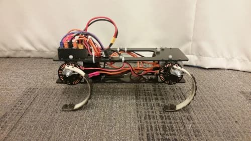
QRHex, shown in Figure 1, is a power- and computation autonomous quadrupedal robot. It is a quadrupedal RHex-style, [20], robot with one actuator per hip powering compliant C-shaped legs.

Mechanical Design

QRHex’s four legged design was influenced by the scaling arguments developed in [11]. These imply that specific force for a fixed mass budget scales as $n^{-1}$, where $n$ is the number of actuators. This suggests that, for a RHex-style direct drive robot, a quadruped can be more torque efficient than a hexapod. See Table I for detailed specifications.

Table 1. DIMENSIONS

Let to Let Width	25 cm
Body Width	15 cm
Hip to Hip Length	36 cm
Body Height	10 cm
Hip Height	5 cm
Motor Module Mass	0.4 kg
Battery Mass	1.0 kg
Total Mass (with battery)	4.225 kg

Direct Drive

QRHex was built using RHex's compliant, C-shaped, fiberglass legs and the direct-drive infrastructure described in [11]. Each leg is individually actuated by a T-Motor U8 [2], whose position is controlled using the closed loop infrastructure described in [11]. The direct-drive infrastructure allows QRHex to be lighter, more robust to impacts, and mechanically more efficient due the absence of gear related friction [11].

Parameter Space

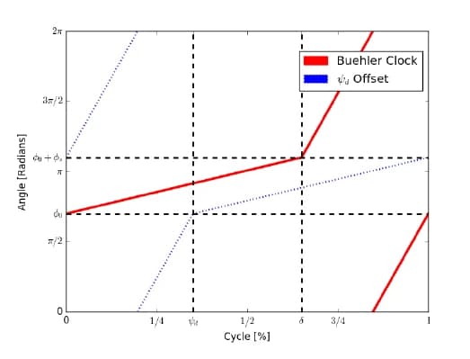
The desired joint angle for a given leg is determined by a Buehler clock [20], depicted in Figure 2. Each leg trajectory is composed of a slow stance phase and fast re-circulation phase of rotation. Within a cycle, the length of the slow section is defined by $\delta \in [0,1]$. This slow section begins at an offset angle ${\varphi }_0\in [0,2\pi ]$ and sweeps for ${\varphi }_s\in [0,2\pi ]$ radians. Each leg $l$ can be at a shifted phase in the cycle relative to a base leg; this is defined by ${\varphi }_{d,l}\in [0,2\pi ]$ in Figure 2. The frequency at which the leg rotates about the hip is denoted $\omega \in R_{+}$. For the work presented here, the angular frequency $\omega$ was held constant and the phases ${\varphi }_{d,l}$ locked in a bound such that the front two legs were $\pi$ radians offset from the back. We denote the remaining set of parameters by $\theta \in B\subset {\mathbb{R}}^5$. We denote the $i^{th}$ parameter by ${\theta }_i$ and the upper and lower bounds on its value by ${\bar{\theta }}_i$ and ${\underline{\theta }}_i$, respectively. The leg joint angle is driven to follow the Buehler clock nominal trajectory using a PID control; the PID control gains were tuned separately and held fixed throughout the work reported here.

Experimental Setup

This work required that trials be run on both on a physical machine and on a simulated construction of that machine.

Vicon

During a given trial we used a Vicon camera setup in an 8 by 20 meter corridor to collect the ground truth position and orientation of QRHex [4]. The system operated at an update frequency of 100Hz and published data to a ROS node for later analysis [1]. Each trial consisted of running the robot for 30 seconds on a given gait. Through empirical testing we determined that an expert operator could significantly narrow down the gait space to an admissible subset from 30 randomized gait trials. Thus we aimed to develop learning algorithms.

Simulation

Because trials are costly in time and wear out the robot, a simulation was designed to estimate gait costs. Due to the complexity of the system a high fidelity model is challenging to create. For example, compliant C-shaped legs are notoriously difficult to model [6], motor performance changes as the actuators heat up, and slight adjustments to the battery position alter the natural frequency of the robot’s pitching dynamics. Because of this, a crude representation of the robot was constructed in the Unity physics engine [3] by defining the leg to be a rigid body constrained to parasagittal planes on either side of the robot. Each leg experiences a restoring force in the plane from a spring with rest length zero (See the supplementary video). Let $\gamma \in {\mathbb{R}}^4$ denote the simulation parameters: spring stiffness, joint damping, maximum joint force, and leg mass. To calibrate the values of $\gamma$, a small set of randomized trials, denoted $\Theta$, was used to minimize the difference between the robot and the simulation. Let $C(\theta )$ define an arbitrary cost function (the specific cost function used will be defined in the following section). First the set of gaits, $\Theta$, was run on the physical machine and the costs recorded. Then the same gaits were run on the simulation over a brute force selection of simulation parameters. The value of $\gamma$ was determined using the least squares method.

${\gamma }^{\ast }={\min }_{\gamma }{\sum }_{\theta \in \Theta }(C_{sim}(\theta )-C_{phys}(\theta ){)}^2$

Cost Function

The standard cost function used in the RHex literature is the cost of transport, measured by specific resistance or speed-weighted specific resistance [21], [9]. However, measuring specific resistance requires specialized hardware in order to get accurate measurements of the energy consumed by a given gait. This hardware is costly and was not readily available as part of the QRHex electronics infrastructure, so we sought to determine a new definition of a “good” gait, i.e., a proxy for specific resistance. The form of this new cost function rewards periodic motion while seeking gaits inherently robust to noise. Even when it is available, the energy measurement hardware is expensive, so the new definition is likely to be useful for applying online gait learning techniques to other low-cost legged robots.

The specific resistance data we provide was calculated using the energy discharged from the battery averaged over long trials and so the cost per trial is an order of magnitude greater than our new cost function. Because of these high costs per trial, it is infeasible to use this measurement technique for the learning process and so we use it only to validate the efficiency of the learned gaits.

As defined above in Section II-C, let $\theta$ be the set of variable parameters that determine a gait. We have set $\theta$ to be the duty cycle, sweep, and offset of a Buehler clock (other Buehler clock parameters are held constant). Let $\omega$ be the driving frequency of the gait.

Let $z(t;\theta )$ be the height of the vehicle relative to the ground as a function of time $t$ for a trial with a given parameter value $\theta$. We will consider the frequency content of the signal $z$, which we expect to be concentrated around harmonics of the driving frequency $\omega$. Through extensive use of this machine we have noticed gaits that we deem “good” excite multiples of the driving frequency as seen in Figure 3. Furthermore, gaits that exhibited these harmonic structures tended to have lower specific resistances. It should be noted that the lack of this structure gave no indication as to the efficacy of the gait. This leads us to believe that our cost function is a suitable proxy for a subset of the specific resistance. We quantify this notion of “goodness” using the Fourier transform of $z$. Let $Z(k;\theta )$ be the Fast Fourier Transform (FFT) of the discretely-sampled time series $z(t;\theta )$ and let $f$ be a small frequency window strictly less than the driving frequency $\omega$.

We define the function $S(\theta )$ as a measure of how much structure is present in the FFT in hopes that this demonstrates that the algorithm is learning and utilizing the natural mechanics of the robot. Let N be the number of harmonics considered. We have seen through experimentation that at higher frequencies the amplitude of a peak in the FFT decreases to the point where it becomes indistinguishable from noise and so, only a few harmonics need to be considered. We have set N = 10. Let $S(\theta )$ be defined as follows:

$S(\theta )={\sum }_{n=1}^N\frac{{\max }_{[n\omega -f,n\omega +f]}(Z[k,\theta ])}{{\text{mean}}_{[n\omega -f,n\omega +f]}(Z(k,\theta ))},$

where the subscripts define the intervals over which the means and maxima are computed. The function $S$ compares the peak values of the FFT against the means of a small interval situated around the first N harmonics. The better defined the peak around a given harmonic, the larger its contribution to the function value. Note that the function $S$ is real-valued and positive.

Let ${\mu }_{\theta }$ be define as the average ground speed for a given set of gait parameters. Let $\alpha \in [0,1]$ be a tuning constant that trades off between speed and harmonic structure. The total reward function $R(\theta )$ is defined as follows:

$R(\theta )=(1-\alpha ){\mu }_{\theta }+\alpha H(\theta )$

Minimizing a cost $C(\theta )$ is equivalent to maximizing the reward $R(\theta )$. We can define the cost $C(\theta )$ of a gait as the negative of the reward, as we prefer to follow the convention in the optimization literature of minimizing costs.

$C(\theta )=-R(\theta )$

In this work we measure $z$ using the Vicon system, but we hypothesize that $Z$ could be effectively estimated using an accelerometer on board the robot.

ALGORITHMS

We compared the performance of three different optimization algorithms: Nelder-Mead, Simulated Annealing, and the Upper Credible Limit (UCL) algorithm from the multi-armed bandit literature. UCL is a Bayesian algorithm that can use informative priors to improve its convergence rate. We used data from simulated experiments to develop priors for UCL. These priors also provided the initial conditions for the Nelder-Mead and Simulated Annealing trials.

Nelder-Mead

In the past, Nelder-Mead has been used for gait optimization on RHex-like machines, see [21]. Nelder-Mead is a local optimization algorithm that is often effective despite the fact that it can fail to converge to local optima [14]. Because it is a local algorithm, the results of employing Nelder-Mead depend strongly on the initial conditions. Nelder-Mead was tested twice utilizing the gaits with lowest cost found by the simulation as initial conditions.

Simulated Annealing

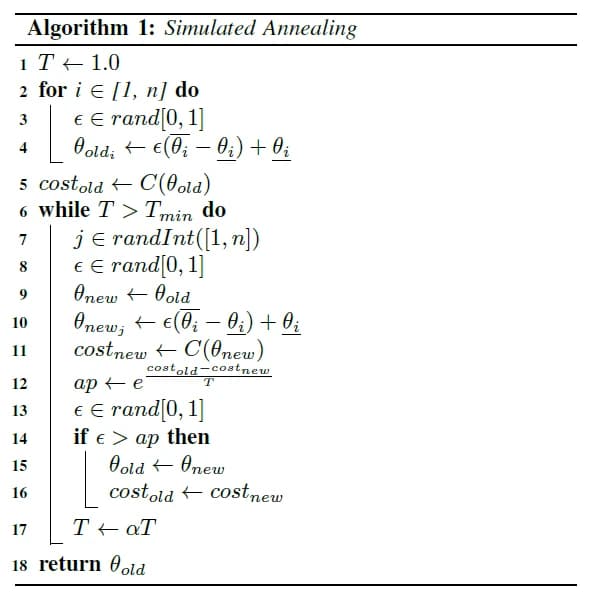
Because Nelder-Mead is a local optimization technique we also tested a global optimization algorithm, namely, Simulated Annealing [12]. See Algorithm 1 for the pseudocode of the algorithm we implemented. Similarly, the initial gait was selected from the simulation results. Recall that $\theta$ is the set of gait parameters. We define the current best set of parameters and the respective cost as ${\theta }_{old}$ and $cos{t}_{old}$. The next gait to test and its cost are then denoted by ${\theta }_{new}$ and $cos{t}_{new}$. We define $T$ to be the current temperature of the system, $T_{min}$ to be the stopping condition, and $\alpha$ to be the rate of cooling. We declared $T_{min}$ = 0:05 and $\alpha$ = 0:87 for our trials. We define $ap$ to be the $acceptanceprobability$, the chance we switch to a lower cost gait.

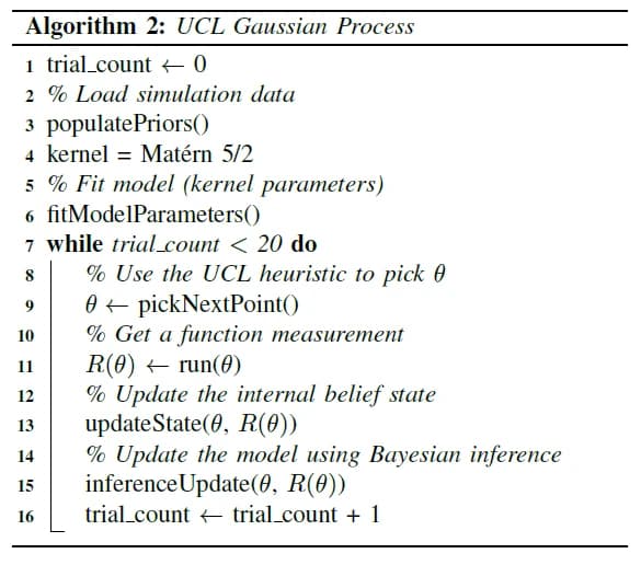
UCL Gaussian Process

As noted in the introduction, empirical measurements of gait quality on QRHex are corrupted by significant noise. Therefore, we tested an implementation of the UCL algorithms developed in [19], [18]. These algorithms perform Bayesian optimization on discrete spaces and admit performance guarantees that show that they converge to the global optimum at a maximal rate.

As a Bayesian algorithm, the performance of UCL can be strongly affected by the choice of priors. Furthermore, standard UCL operates on a discrete space, while the gait parameter space $B$ is continuous. Therefore, two challenges that had to be addressed in implementing UCL for our system were the discretization of the parameter space and generating priors over the cost $C$. For this initial work we discretized the space $B$ using a uniform rectangular grid and adjusted the granularity of the discretization for each parameter to find a reasonable compromise between grid resolution and the number of grid points. It should be noted that Nelder-Mead and Simulated Annealing were implemented in their standard forms, operating on the continuous domain $B$.

As noted above, we developed priors over this discrete space using simulation data. All three algorithms used these priors to seed their initial conditions. A key feature of thec ost function is that it appears to be continuous, so it is natural to use kernels to represent the dependencies among the function values at different points. We used the Python module GPFlow [17], which implements many different standard kernels, to implement the priors and perform the Bayesian updates. Through experimentation, we found that the Mat´ern 5/2 kernel resulted in the best performance, likely because it models a reasonable amount of smoothness in the cost function. See Algorithm 2 for details of the implementation of UCL we used in this work.

RESULTS

We present data from several series of learning trials performed on the physical robot and show that, while each optimization algorithm achieved some improvement in the gait, the UCL algorithm achieved greater and more consistent gains.

Regret

We present the results of the learning process in terms of regret [19], which is commonly used in the multi-armed bandit literature to measure performance. The regret of a choice is a measure of how much more costly that choice is compared to the best choice that could have been made. To measure regret in an empirical setting one must choose an estimate of the best possible choice, which sets the reference value for measuring regret. Because each gait has a deviation in costs associated with it, it is possible that a gait with high average cost could achieve the absolute minimum cost during any given trial. This, however, will not yield an optimal solution over many trials and so we defined the regret from the minimum average cost, $\bar{C}$. Let ${\theta }^{\ast }$ be the parameter set that yields the lowest average cost. Thus regret from trial $t$ is defined as:

${\hat{R}}_t=\bar{C}({\theta }^{\ast })-C({\theta }_t)$

and the cumulative regret at time $T$ is the sum ${\sum }_{t=1}^T{\hat{R}}_t$ Lower cumulative regret corresponds to faster convergence. From this definition the cumulative regret can decrease but a solution that approaches the optimal gait will still tend to zero slope.

The data presented in Figure 4 shows the total cumulative regret over the course of learning epochs, two epochs for each algorithm studied. Each epoch consisted of only 20 trials as 10 trials were used to calibrate the simulation and it had been determined an expert operator could narrow down the gait space in 30 randomized trials. Trials are scarce as running the physical machine is time intensive.

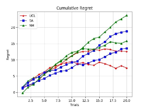
Figure 4 shows both UCL epochs determine the optimal solution in approximately ten trials. Both epochs converged on the same solution further showing the robustness of the algorithm to uncertainty from measurement noise. The Simulated Annealing epochs have close to constant slopes, indicating roughly constant regret ${\hat{R}}_t$. This result could be ascribed to the rapid cooling required to converge the annealing algorithm within the trial limit. While Simulated Annealing has nice global properties it seems ill suited for this particular physical machine where the cost of performing a trial is high. When Nelder-Mead was initialized using the top four gaits provided by the simulation the algorithm converged on a suboptimal local optimum which can be seen as the result with the highest regret in Figure 4. The second Nelder-Mead epoch started with the next four best gaits which included the set of parameters the UCL algorithm converged to. With these initial conditions Nelder-Mead was able to converge on a near-optimum solution. However, even when initially provided with an optimal gait, the convergence is slower than both UCL trials.

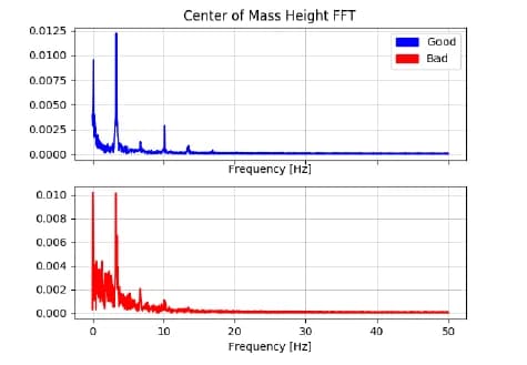
Gait Frequency Content

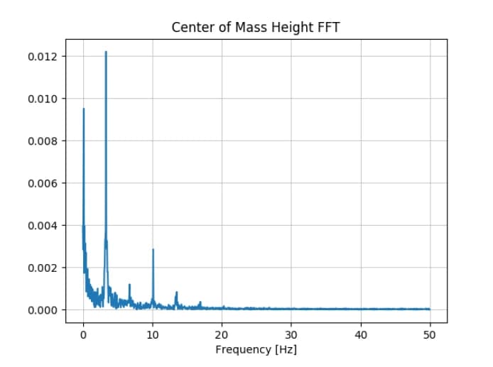
The effect of our cost function can be best seen by comparing the FFT plots in Figure 5 which shows the optimal gait found by UCL and the local optimum found in the first Nelder-Mead epoch. The “good” gait has its frequency content much more cleanly concentrated around the harmonics of the driving frequency. The “good” example is the same data as seen in Figure 3 but is repeated for ease of comparison. The physical differences between the gaits can be better perceived in the supplementary videos.

Specific Resistance

While not directly learning over specific resistance, the minimization of our cost function resulted in a 36.6% decrease in the standard cost of transport as seen in Table II. The second Simulated Annealing epoch, while not performing well on our cost function, resulted in a specific resistance close to that of the UCL algorithm. This provides an example for the observation made in Section IV that the lack of structure in the FFT does not provide information on the efficacy of a gait.

Table 2. SPECIFIC RESISTANCE

Algorithm	Epoch	Starting SR	Ending SR	% Change
UCL	1	5.25	3.33	-36.6%
UCL	2	5.25	3.33	-36.6%
SA	1	5.25	3.72	-29.1%
SA	2	5.35	3.42	-36.2%
NM	1	5.25	4.19	-20%
NM	2	3.33	3.80	+9.0%

DISCUSSION

The work presented here leaves open many avenues of future research. We focused on the learning aspect of this problem but this revealed some interesting mechanical aspects of the system which warrant further investigation. Another interesting direction would be to investigate the use of a physics engine to construct a crude model of the robot and how much information about the physical robot can be gleamed from these simulations.

Buehler Clock

We selected a Buehler clock as the parametric representation of the gait space because it is the representation that is most commonly used in the literature on RHex-type robots. The gaits implemented using the Buehler clock tend to be such that the slow section of the gait occurs during contact with the ground followed by a fast recirculation. However the optimal solution found by the UCL algorithm operates differently: it rotated the slow section well out of ground contact. We believe that, because the space was discretized relatively coarsely, the size of the slow section was used in concert with the duty cycle to adjust the impact velocity between the legs and the ground during the fast phase. Further research can be done by looking into whether replacing control over the duty cycle and sweep size with direct leg recirculation speeds yields similar results on this particular machine.

An additional behavior of the optimal gait is a slight impacting of the tail end of the robot with each step. Some of the gaits tested did not exhibit this behavior and so it was specifically selected. This feature appears critical to the performance; if the base plate of the robot is shortened by an inch the gait looses its stability, see the supplemental video. One potential theory is that this is an artifact arising from the relative impact locations of the front and back legs in relation to the center of mass, similar to the toe stubbing for pitch correction when jumping with RHex [10]. This question warrants further investigation.

Simulation Fidelity and Mechanical Sensitivity

Further research can be done on the tactic of using a crude simulation to generate prior data. While accurate simulations are desirable, the calibration process is susceptible to inconsistencies in the mechanical properties of the robot from trial to trial. For instance, we found that the cost of gaits would change dramatically if the battery position was adjusted by as little as a centimeter. This is likely due to the fact that the battery makes up a large percentage of the robot’s weight, about 24%, and so by shifting the center of mass slightly, one adjusts the natural frequency of the robot’s pitching dynamics. This suggests another optimization problem between the cost of simulation trials versus the cost of physical trials. For instance, the rate of convergence could be explored as a function of the number of trials used to calibrate the computer model.

Trial Length

Another area of investigation would be in testing the relationship between the cost function we defined and the trial length. Longer trials may decrease the impact noise introduced by the legs snapping into position at $t=0$ has on the overall cost of a gait. Thus trials with more clock cycles could reveal efficient gaits that take longer to converge. However, this means that shorter trials could produce slightly less efficient gaits that are more robust to the initial conditions of the legs and quickly fall into a steady state.

CONCLUSIONS

In this paper we compared methods of gait optimization on a RHex-like machine and showed that stochastic algorithms should be considered to account for uncertainties in real-world data. While bandit-style algorithms have been used for gait adaptation on other morphologies, this paper is the first to use the UCL algorithm and the first to do so with the RHex-style morphology consisting of a single actuator per hip with compliant C-shaped legs. We also provided a proxy to specific resistance which we hope to use to explore online learning with cheap legged systems. Looking forward, this work aims to develop rigorous and efficient methods for inexpensive legged robots to actively adapt their gaits to their environment.

ACKNOWLEDGMENT

This work was funded in part by AFRL grant FA865015D1845 (subcontract 6697371). We acknowledge the support of various members of Kod*lab and Ghost robotics in doing this work, as well as Maria Mathew.

REFERENCES

[1] Ros driver for motion capture systems. Online. Available: https://github.com/KumarRobotics/motion capture system.

[2] T-motor u8 datasheet. Online. Available: www.rctigermotor.com/.

[3] Unity physics engine. Online. Available: https://unity3d.com/.

[4] Vicon datasheet. Online. Available: https://docs.vicon.com/download/attachments/25296959/Vicon

[5] P. Auer, N. Cesa-Bianchi, and P. Fischer. Finite-time analysis of the multiarmed bandit problem,. Machine Learning, 47(2/3):235–256, 2002.

[6] Y. Aydin, K. Galloway, Y. Yazicioglu, and D. Koditschek. Modeling the compliance of a variable stiffness C-shaped leg using Castigliano’s theorem. 08 2010.

[7] S. Chemova and M. Veloso. An evolutionary approach to gait learning for four-legged robots. 2004 IEEE/RSJ International Conference on Intelligent Robots and Systems (IROS) (IEEE Cat. No.04CH37566), pages 2562–2567.

[8] A. Cully, J. Clune, D. Tarapore, and J. B. Mouret. Robots that can adapt like animals. Nature, 521(7553):503–507, 2015.

[9] G. Gabrielli and T. von Karman. What Price Speed?: Specific Power Required for Propulsion of Vehicles. 1950.

[10] A. M. Johnson and D E Koditschek. Toward a vocabulary of legged leaping. In Proceedings of the 2013 IEEE Intl. Conference on Robotics and Automation, pages 2553–2560, May 2013.

[11] G. Kenneally, A. De, and D. E. Koditschek. Design principles for a family of direct-drive legged robots. IEEE Robot. Autom. Lett. IEEE Robotics and Automation Letters, 1(2):900–907, 2016.

[12] S. Kirkpatrick, C. D. Gelatt, and M. P. Vecchi. Optimization by simulated annealing. Science, 220(4598):671–680, 1983.

[13] N. Kohl and P. Stone. Policy gradient reinforcement learning for fast quadrupedal locomotion. IEEE International Conference on Robotics and Automation, 2004. Proceedings. ICRA ’04. 2004, pages 2619–2624, 2004.

[14] T. G. Kolda, R. M. Lewis, and V. Torczon. Optimization by direct search: New perspectives on some classical and modern methods. SIAM Review, 45(3):385–482, 2003.

[15] M. A. Lewis and G. A. Bekey. Gait adaptation in a quadruped robot. Autonomous robots, 12(3):301–312, 2002.

16] D. J. Lizotte, T. Wang, M. H. Bowling, and D. Schuurmans. Automatic gait optimization with gaussian process regression. In IJCAI, volume 7, pages 944–949, 2007.

[17] A. G. de G. Matthews, M. van der Wilk, T. Nickson, K. Fujii, A Boukouvalas, P Leon-Villagra, Z Ghahramani, and J Hensman. GPflow: A Gaussian process library using TensorFlow. arXiv preprint 1610.08733, 2017.

[18] P. Reverdy, V. Srivastava, and N. E. Leonard. Satisficing in multiarmed bandit problems. IEEE Transactions on Automatic Control, 2017.

[19] P. B. Reverdy, V. Srivastava, and N. E. Leonard. Modeling human decision making in generalized gaussian multiarmed bandits. Proceedings of the IEEE, 102(4):544–571, 2014.

[20] U. Saranli, M. Buehler, and D. E. Koditschek. Rhex: A simple and highly mobile hexapod robot. The International Journal of Robotics Research, 20(7):616631, Jan 2001.

[21] J. D. Weingarten, G.A.D. Lopes, M. Buehler, R.E. Groff, and D.E. Koditschek. Automated gait adaptation for legged robots. IEEE International Conference on Robotics and Automation, 2004. Proceedings. ICRA ’04. 2004, pages 2153–2158, 2004.

[22] J.D. Weingarten, M. Buehler, R.E. Groff, and D.E. Koditschek. Gait generation and optimization for legged robots. In The IEEE International Conference on Robotics and Automation, 2002.